Fractal trees: Recursion, quaternions and optimization.
More than an article or a blog, this is a journey. A journey without a final destination — just learning. In which fractal trees are just the ship. The truly valuable objective is all the cool things we will learn by riding it.
So … with that out of the way, get a cup of your preferred beverage and let’s begin!

My preferred beverage is vodka.
I don’t know about that Ratalf, I was thinking about something more like tea or coffee. But okay, we need to continue.
We will start by making a simple 2D fractal tree.
To do it we need two simple tools:
- Some way to construct finite lines in 2D space.
- Some way to rotate, translate, and scale such lines.
I have an idea!! Let us represent lines with two points. The beginning and the end of the line. And maybe we can use some vector tricks to rotate, translate and scale the line.
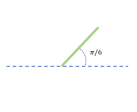
Everything starts with a single line, a point at the origin and one at .
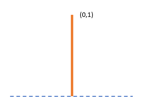 |
|---|
If a line starts at the origin we can think of it as a vector. Therefore we can use cool linear algebra techniques to scale and rotate this vector. Just keep this in mind for later.
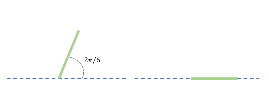
Now let’s grab our line and clone it two times. And we also want the clones to be a little smaller than the original — let’s say 0.7 times the original size.
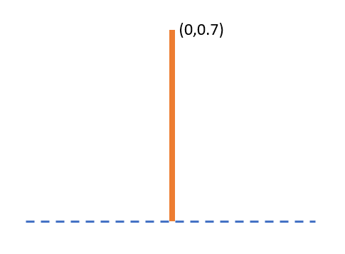 |
|---|
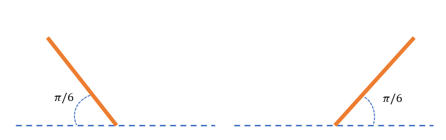
Then we want to rotate both of them by an angle with respect to the parent, one to the left and one to the right.
Easy!! We can use a rotation matrix.
Yeah, that’s an option, but I have a better idea. Complex numbers!!
Whenever we are working with rotations in 2D space it is very convenient to work with complex numbers. In fact, for this application, we can think about complex numbers almost the same as we think about vectors.
Instead of having a vector we have .
But why use complex numbers?
Well, many reasons, but the most important here is that complex numbers are commutative, that is:
This property gives us a convenient way to rotate a vector with a simple “multiplication”. Imagine we want to rotate the vector by radians. With a rotation matrix, we will need to do this:
The same operation with complex numbers looks like this:
At the end, both methods are computationally equivalent, but the complex number one is cleaner. And it gets better if we introduce Euler’s identity.
Tell me that’s not clean as heck.
Yeah, yeah it's kind of neat.
Okay now, let’s get back to our lines. We have the parent line represented by the complex number , and because the line starts at the origin, we can think of the line just as alone.
Then we make two copies:
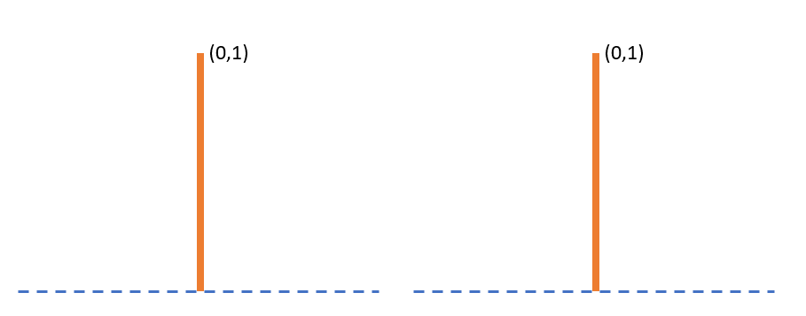 |
|---|
Scale them by 0.7
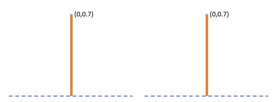 |
|---|
Rotate each child line by
 |
|---|
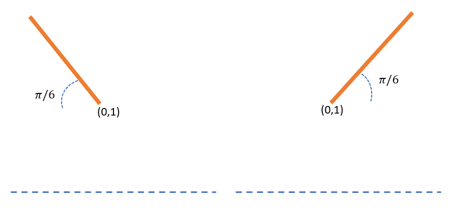
Finally, we translate the beginning of each line by the end of the parent line.
 |
|---|
Therefore the beginning of our child lines would be the end of the parent line.
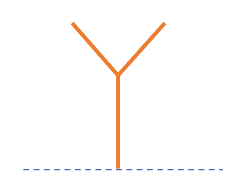
Bring It all together and we have our first two-branched tree.
 |
|---|
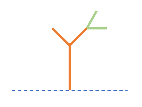
Now, we repeat the same procedure but for the child lines. The only new condition is that before rotating and scaling we need to move the line back to the origin — in order to treat the line as a single complex number. That is as easy as subtracting the beginning to the end of the line. And we already know that the beginning of the child line is the end of the parent line.
Just for clarity, let’s make one more iteration for the right branch.
Focusing on the right branch. First, we move it back to the origin by subtracting the parent line.
 |
|---|
We make two copies, and scale them by the scaling factor . And rotate each child by
 |
|---|
Finally, we move the beginning of each line to the end of the parent line.
 |
|---|
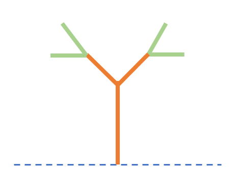
If we do the same with the left branch, we would have a fractal tree with a recursive factor of 3.
 |
|---|
Now that we understand the math, we can code it. You probably already have some ideas — this is clearly a recursive process. And also, we can imagine that somehow this process needs to be repeated for the left and right branches. But first, we need a function to draw lines where the input is two complex numbers.
Pythondef plot_complex(origin, end):
    x = [origin.real, end.real]
    y = [origin.imag, end.imag]
    plt.plot(x,y, linewidth = 3
Now, think about the actual recursive function. We already know the steps of the algorithm — also the parameters we need.
The parameters:
- initial line.
- rotating angle.
- scaling factor.
- number of generations of branches (recursion factor).
In code:
Python#initial line
origen = 0 + 0j
end = 0 + 1j

angle = math.pi / 6
scale = 0.7
recursion_factor = 11
The steps:
- Clone parent line
- Move it back to the origin.
- Scaling the lines.
- Rotate lines.
- Move them back to the end of the parent line.
- Repeat for child lines.
In code, thanks to complex numbers we can do most of the steps in a single line, at least 2 to 5:
Pythondef tree(origin, branch, angle, scale, rec_factor):
    if rec_factor > 0:
        plot_complex(origin,branch)
        branch_l = ((branch-origin) * e ** (1j*anglel)*scale)+branch
        branch_r = ((branch-origin) * e ** (-1j*angler)*scale)+branch
        tree(branch,branch_l,angle,scale,rec_factor-1)
        tree(branch,branch_r,angle,scale,rec_factor-1)
Test.
Finally, we can run the function:
Pythonorigin = 0 + 0j
first_end = 0 + 0.7j
angle = math.pi / 6
scale = 0.5
recursion_factor = 12

tree(origin, first_end, angle,scale,recursion_factor)
plt.show()
 |
|---|
Cool!!
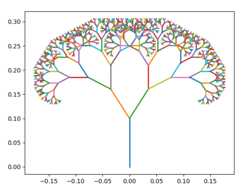
Now that we have the basic algorithms. We can have some fun. Maybe adding some color dependence on the recursive factor, and different angles for left and right branches.
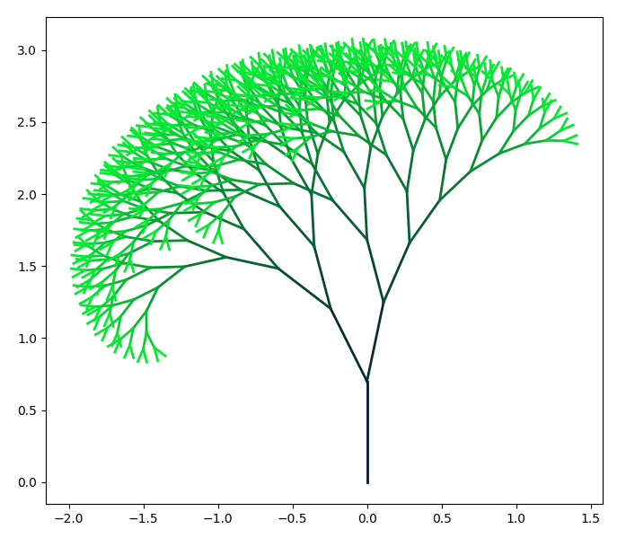 |
|---|
Pretty, isn’t it?
You can do so much more. Have fun!! Be creative. I swear, I can spend countless hours trying to come up with a beautiful fractals tree.
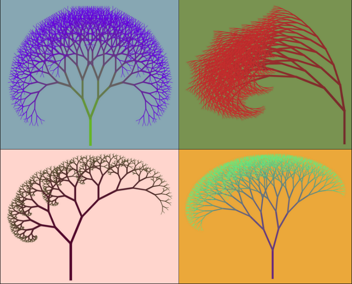 |
|---|
But be careful. You don’t want to go wild with the recursive factor. You probably already notice this is an algorithm.The exact number of branches is:
Where is the number of generations or recursive factor.
| n | lines |
|---|---|
| 1 | 1 |
| 2 | 3 |
| 3 | 7 |
| : | : |
| 11 | 2047 |
| 12 | 4095 |
Yes, the number of branches grows super fast. Probably, going much higher than 16 is a bad idea — if you value your poor computer.
Now the fun begins!! Let’s go up a dimension!!!!
Oh crap, I hate y'all three-dimensional beings.
We already know how to construct a fractal tree in 2D. Going up a dimension should be straightforward.
But guess what?… There are also two options.
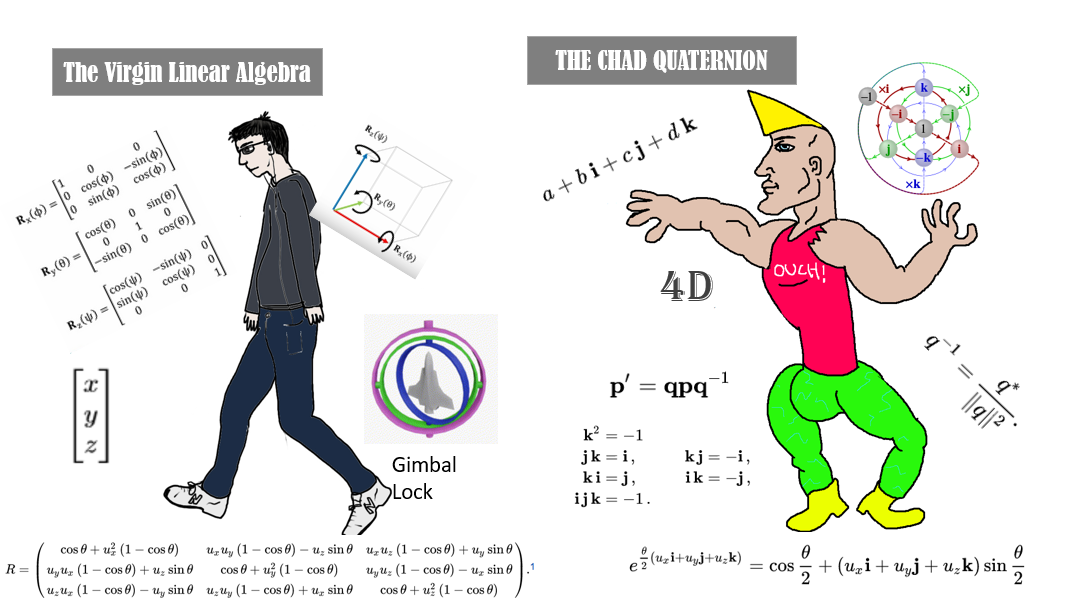 |
|---|
I don’t know about you, but I’m all about higher dimensional number systems. Quaternions are the option for me.
Wait!! "quat" means four "thingies", doesn't it?
Yep, quaternions are a four-dimensional number system.
But we only need 3 dimensions. Why don't we use “threeternions” or whatever they are called?
Short answer, they do not exist. In fact, it is impossible to create a 3-dimensional number system. For some fancy math reasons there is no algebraic coherent triplex, and quaternions are the next best thing.
But trust me, do not be intimidated by the extra dimension. For our purposes, we can mostly ignore it. You will see!
Okay, but two questions. What the hell are quaternions? And why quaternions?
You can think of quaternions as an extension of complex numbers to four dimensions. But unlike complex numbers, quaternions are a bit weirder to work with. But they have some advantages over using rotation matrices in 3d (For example lack of gimbal lock).
Quaternions are defined by one real dimension and 3 “imaginary” dimensions.
Unlike complex numbers, quaternion multiplication is non-commutative. Which makes them a little harder to work with. But we have computers. If we know the rules and how to code them, we can let the computer do the hard stuff.
Let us start with the multiplication of the basis. This is a handy table:
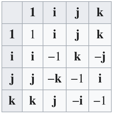 |
|---|
If you stare at the table for a few seconds, you can see why quaternion multiplication is non-commutative. For example but . That is why from now on, we will have to be more careful with the multiplication order.
That little table is the hardest part. The multiplication of two arbitrary quaternions follows the good old distributive law you are already know from high school — with the only catch of being aware of the order.
By grouping by the basis:
To perform rotations with quaternions, we also need the quaternion inverse. It is quite straightforward:
Let be an arbitrary quaternion , is the inverse of if . The inverse is constructed by.
One more thing. The same way we use Euler’s identity with complex numbers, we can define an analog exponent for quaternions.
Where is a unit vector.
Finally, we have all the pieces to construct 3d rotation with quaternions.
A little counterintuitively we will use the three imaginary dimensions of quaternions , to represent the three spatial dimensions. The real part of the quaternion is only used in the arithmetic operations (For this use case). So, the representation of a vector in 3D space with quaternions looks like:
Let’s say we want to rotate a point in 3d space around the axis defined by a unit vector by radians. Hear me out, this will seem a little bit weird at first, but I promise it makes sense. The operation would look something like this:
Wut?
Told you… but we can try to understand it. We need to keep in mind is that quaternion multiplication are in fact 4-dimensional rotations. That’s why we need to also multiply by the inverse. The easiest way to understand it is to play with an interactive quaternion plotter. But in essence, you can think about the operation as first making a 4D rotation of radians around the defined axis with . Then we multiply by to counteract the contribution of the fourth dimension and rotate the point the extra that remains. That’s why we have to divide by 2 in the exponent. his fact is
So, basically is a trick to construct 3-D rotations with 4-D operations
Yeah! that’s basically it.
Finally, we have everything to start codding again.
I can help but panic a little. I know for a fact that python doesn't have support for quaternions. Just saying.
Piano piano, don’t rush Ratalf. There are many possible solutions. Just a quick recap of everything we need in code:
- Some representation quaternions in code.
- Some way to do algebraic operations with quaternions.
- A plotting function.
For the first requirement (quaternion representation) we have multiple options. We would use a python library that supports quaternions — Numpy quaternion for example . Which would also solve the second requirement (algebraic operations), killing two rats with one stone.
rude
Another option is to use tuples or arrays to represent quaternions, then write functions for each algebraic operation. For example:
Pythondef sum_quaternion(a: tuple,b: tuple):
  return (a[0]+b[0],a[1]+b[1],a[2]+b[2],a[2]+b[3])
I like this approach more because it is more DIY — and not overkill as Numpy quaternion. But, chaining multiple algebraic operations would rapidly become really clumsy.
Pythona = (1,2,3,4)
b = (5,6,7,8)
c = (9,10,11,12)
d = (13,14,15,16)
#compute sum_qut = a+b+c+d
sum_quat = sum_quaternion(sum_quaternion(sum_quaternion(a,b),c),d)
That's ugly AF! I just wish we could use simple math operators like + or *.
You hit the nail on the head dear Ratalf. With the magic of python classes and dunder methods, we actually can use math operators. In fact, I think this is the perfect example to understand dunder methods.
Dunder methods also called magic methods, are special types of methods in python that begin and end with a double underscore. This methods allows user-defined classes to use built-in operators and functionality of python. This is called operator overloading. These special methods are the reason why we can sum two strings 'string1'+'string2'. If we define a consistent addition operation between two objects, we can use the dunder method __add__, to then be able to use the plus operator to make an “addition” between them.
If you have coded any amount of Object-Oriented python, you must already know about the dunder method __init__ — the “constructor”, which simplifies the creation of new objects. But there are many more magic methods.
Quaternions are useful for much more — not only rotations. So, I believe is a good idea to make a small separate quaternion module.
Bash$touch quaternion.py
This module will contain the Quaternion class.
Pythonclass Quaternion:
    def __init__(self, w, i, j, k):
        self.w = w;
        self.i = i;
        self.j = j;
        self.k = k;
Now, we can start adding some methods to our class. Starting with addition and subtraction.
Python    def __add__(self,q): # Adds this quaternion with another q quaternion.
        return Quaternion(self.w+q.w,self.i+q.i,self.j+q.j,self.k+q.k)
    def __sub__(self,q): # Substracts this quaternion with another q quaternion.
        return Quaternion(self.w-q.w,self.i-q.i,self.j-q.j,self.k-q.k)
Then scalar multiplication. For simplicity, I decided to use the * operator only for scalar multiplication.
Python    def __mul__(self,c): # Multiply this quaternion with a constant "c"
        return Quaternion(self.w*c,self.i*c,self.j*c,self.k*c)
And the @ operator, with dunder method __matmul__ for quaternion multiplication.
Python    def __matmul__(self,q): # quaternion multiplication
        a0, a1, a2, a3 = self.w, self.i, self.j, self.k
        b0, b1, b2, b3 = q.w, q.i, q.j, q.k
        return Quaternion((a0*b0-a1*b1-a2*b2-a3*b3),(a0*b1+a1*b0+a2*b3-a3*b2),(a0*b2-a1*b3+a2*b0+a3*b1),(a0*b3+a1*b2-a2*b1+a3*b0))
That’s all we need. But since we are already here, we might as well add some quality of life methods. Starting with __iter__ — a quite useful method.
Python    def __iter__(self):
        return iter((self.w,self.i,self.j,self.k))
It allows the use of quaternions as iterators, and do cool things like:
Pythona,b,c,d = Quaternion(1,2,3,4)
print(a) # 1
Test.
Wow!
Maybe absolute value would also be handy.
Python    def __abs__(self):
        return sqrt(self.w**2+self.i**2+self.j**2+self.k**2)
And __str__ is always a good idea, it gives Quaternion a string representation.
Python    def __str__(self):
        return f'[{self.w},{self.i},{self.j},{self.k}]'
Now we can print quaternions by just:
Pythonq = Quaternion(1,2,3,4)

print(q) # [1,2,3,4]
Finally, the only not dunder method that we need. The quaternion inverse:
Python    def inv(self):
        c = 1/abs(self)
        return Quaternion(self.w,-self.i,-self.j,-self.k)*c
Look!, we already use some of our special methods.
That’s it!. That right there is our small quaternion module.
Pythonclass Quaternion:
    def __init__(self, w, i, j, k):
        self.w = w;
        self.i = i;
        self.j = j;
        self.k = k;

    def __add__(self,q): # Adds this quaternion with another q quaternion.
        return Quaternion(self.w+q.w,self.i+q.i,self.j+q.j,self.k+q.k)
    def __sub__(self,q): # Substracts this quaternion with another q quaternion.
        return Quaternion(self.w-q.w,self.i-q.i,self.j-q.j,self.k-q.k)
    def __mul__(self,c): # Multiply this quaternion with a constant "c"
        return Quaternion(self.w*c,self.i*c,self.j*c,self.k*c)
    def __str__(self):
        return f'[{self.w},{self.i},{self.j},{self.k}]'
    def __iter__(self):
        return iter((self.w,self.i,self.j,self.k))
    def __abs__(self):
        return sqrt(self.w**2+self.i**2+self.j**2+self.k**2)
    def __matmul__(self,q): # quaternion multiplication
        a0, a1, a2, a3 = self
        b0, b1, b2, b3 = q
        return Quaternion((a0*b0-a1*b1-a2*b2-a3*b3),
                            (a0*b1+a1*b0+a2*b3-a3*b2),
                            (a0*b2-a1*b3+a2*b0+a3*b1),
                            (a0*b3+a1*b2-a2*b1+a3*b0))
    def inv(self):
        c = 1/abs(self)
        return Quaternion(self.w,-self.i,-self.j,-self.k)*c
Now we can start with the 3D fractal trees script.
Bash$ touch 3d_tree.py
Of course we need to import the Quaternion class we made. And also matplotlib for plotting.
Pythonimport matplotlib.pyplot as plt
from mpl_toolkits.mplot3d import Axes3D
import math
from quaternion import Quaternion
To plot in 3D, we can make a 3D projection like this:
Pythonfig = plt.figure()
ax = fig.add_subplot(111, projection='3d')
Now, the plotting function that takes two quaternions, taking the imaginary dimensions from each one as a point in 3D space, and plots a line between the points.
Pythondef plot(q1: Quaternion,q2: Quaternion):
    _, x1, y1, z1 = q1
    _, x2, y2, z2 = q2
    ax.plot([x1,x2],[y1,y2],[z1,z2],linewidth = 3)
Note that the _ signifies that the function do not use the real part of the quaternions.
We also need the previously mention quaternion exponent.
Pythondef quat_exp(theta,vec):
	imag = Quaternion(0,*vec)*math.sin(theta)
	real = Quaternion(math.cos(theta),0,0,0)
	return imag + real
Now we have everything we need to do 3d fractal trees.
... About time.
First, a 2D tree in 3D space. In other words, every branch has only two children — same as the 2D version. But now we have to choose the axis of rotation. For starters, we can choose i.e the axis. For the direction of rotation, you can use the good old right-hand rule.
Pythondef tree(origin,end,scale,angle,rec_factor):
	plot(origin,end)
	if rec_factor > 0:
		exp_lef = quat_exp(angle/2,(1,0,0))
		exp_right = quat_exp(-angle/2,(1,0,0))
		left = (exp_lef@((end-origin)*scale)@exp_lef.inv())+end
		right = (exp_right@((end-origin)*scale)@exp_right.inv())+end
		tree(end,left,scale,angle,rec_factor-1)
		tree(end,right,scale,angle,rec_factor-1)

origin = Quaternion(0,0,0,0)
end = Quaternion(0,0,0,1)

angel = math.pi / 9
scale = 0.7
rec_factor = 9

tree(origin,end,scale,angel,rec_factor)

#limits the plotting space
ax.set_xlim3d(-2, 2)
ax.set_ylim3d(-2, 2)
ax.set_zlim3d(0, 3)

plt.show()
 |
|---|
Lame! That's the same as before.
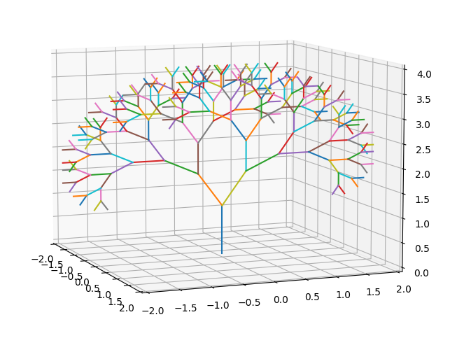
I know, calm down, it’s just a test. Now we can start having some fun. Maybe start with 3 children per branch at radians from each other. The rotation axis are .
Pythondef tree(origin,end,scale,angle,rec_factor):
	plot(origin,end,rec_factor)
	if rec_factor > 0:
		exp_1 = quat_exp(angle/2,(0,1,0))
		exp_2 = quat_exp(angle/2,(-0.866025,-0.5,0))
		exp_3 = quat_exp(angle/2,(0.866025,-0.5,0))
		branch_1 = (exp_1@((end-origin)*scale)@exp_1.inv())+end
		branch_2 = (exp_2@((end-origin)*scale)@exp_2.inv())+end
		branch_3 = (exp_3@((end-origin)*scale)@exp_3.inv())+end
		tree(end,branch_1,scale,angle,rec_factor-1)
		tree(end,branch_2,scale,angle,rec_factor-1)
		tree(end,branch_3,scale,angle,rec_factor-1)

origin = Quaternion(0,0,0,0)
end = Quaternion(0,0,0,1)
angel = math.pi / 6
rec_factor = 7
scale = 0.8

tree(origin,end,scale,angel,rec_factor)

#limits the ploting space
ax.set_xlim3d(-2, 2)
ax.set_ylim3d(-2, 2)
ax.set_zlim3d(0, 3)
plt.show()
 |
|---|
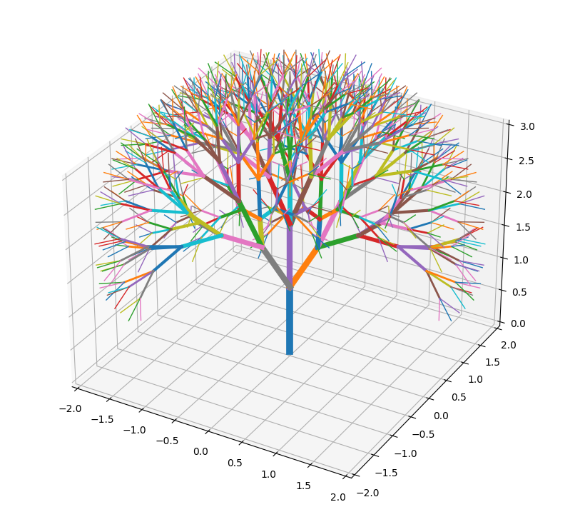
Adding some color, in the plotting function.
 |
|---|
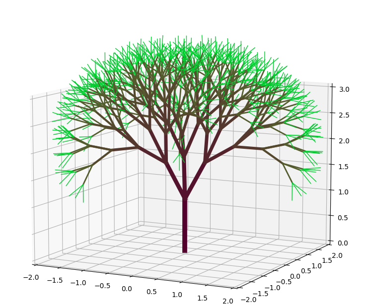
Maybe some extra condition in the plotting function to color the last generation with a different color to simulate leaves.
Okay, okay ... that's beautiful
Told you!! And you can do so much more with this. Have fun!!. Here some of my experiments.
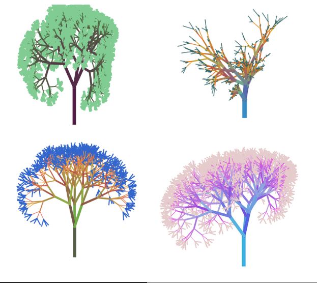 |
|---|
Finally, is a fun exercise to list some thing that we learned in this journey:
- 2D rotations.
- Complex numbers.
- Recursion.
- 3D rotations.
- Quaternions.
- Python Classes.
- Python dunder methods
That was quite the ride
I hope you had fun learning about all this.
Until next time.
I’m saying the hell with all things that used to be
I get into trouble and I hit the wall"
- Bob Dylan